Technical Articles and Product Descriptions

Reference Materials

Additional Products

Race Engine Technology Magazine

INTRODUCTION

Engineers, developers and students of reciprocating engines have been curious about the instantaneous value of cylinder pressure relative to crankshaft rotation since the days in which the pressure in the cylinders was produced by the injection of  superheated steam.

In the days of the steam engine, engineers devised a mechanical recording system which consisted basically of a recording drum which rotated in sync with the output shaft, and a recording pen which traversed axially across the drum in response to actual cylinder pressure.

The measurement of the instantaneous cylinder pressures in internal-combustion piston engines, both spark-ignition and compression-ignition, presents a much more difficult problem, due both to the much higher speeds involved, and to the substantially more harsh (temperature and pressure) environment.

The earliest workable system to measure instantaneous cylinder pressure was an ingenious electromechanical device that used a spark discharge through a graphing paper. The system caused a spark to occur at a preset cylinder pressure, and the preset was manually changed throughout the test, which provided a map of the in-cylinder pressure at each crank angle. But since the mapping took place over an extended number of cycles, it also showed the range of pressure variation from cycle to cycle.

This system is described in detail in Volume 1 of Dr. C.F Taylor's Magnum Opus (ref 5:2:114-119).

An example of the output of that system is shown below in Figure 1 (copied from the above reference volume). The pressure trace line is a series of the small pinprick dots caused by the electric spark marking mechanism.

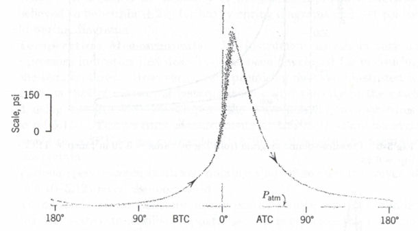
Figure 1: early Combustion Analysis

Figure 1 demonstrates that it has been known for decades that the power produced by a given cylinder in an internal combustion piston engine varies substantially from one cycle to the next.

It follows from that knowldge that, in a multi-cylinder engine, the power produced by each cylinder in the engine differs from the others.

The availability of that knowledge would naturally cause one to wonder how much more power might an engine produce (a) if all the cylinders could be made to operate consistently at their best level from cycle to cycle, and (b) if all the cylinders could be made to operate at the same level as the best one.

The instantaneous values of temperature and pressure in the combustion chamber and in the ports behind the intake and exhaust valves tell volumes about why the engine is performing as it is, and more importantly, suggest ways to make the performance better.

The value of the knowledge contained in the instantaneous pressure information has provided strong motivation for engineers to devise faster and more accurate methods for the substantial challenge of gathering and processing this raw data.

This article attempts to describe the methods by which this instantaneous pressure information is captured and reduced, and the improvements in engine performance which can be obtained through the proper use and application of that information.

HISTORY

In the days before today's sophisticated combustion analysis, and before there were 50 or 70 British Engineers wandering around NASCAR engine shops, the engine developers were well aware of the opportunities that accrued from optimizing cycle-to-cycle and cylinder-to-cylinder performance, but did not have access to the actual data with which to work.

Their method treated the engine as a black box whose inputs are fuel and air and whose outputs are shaft power and heat. The process consisted of (a) deciding on an experiment to try, (b) fabricating the hardware to test the theory, (c) building the engine that incorporates the test hardware and / or configuration, (d) dynamometer testing the engine, and (e) studying the dyno results to evaluate the gain or loss. That is an iterative methodology that requires good design of experiments, and is based on trial-and-error testing that is painfully slow and very expensive.

Here is an example.

In the old days of the Gen-1 small block Chevy (SB1), the intake ports for two adjacent pairs (front pair, rear pair) of cylinders were immediately adjacent to each other, separated by a relatively thin (3/8 inch) wall. The head layout was such that the front two cylinders in the head were mirror images of each other, as were the rear two cylinders. That produced a valve sequence of E-I-I-E-E-I-I-E.

What that did was to (a) place the exhaust valves of the center two cylinders right next to each other, creating a very hot spot in the bridge between those center cylinders, and (b) the E-I-I-E-E-I-I-E valve layout generated dramatically different mixture motion between the front and rear cylinders on a bank and the center two cylinders on a bank.

Visualize how the front two intake runners (on a central 4-barrel manifold) curve down from the plenum to the cylinder head. The runners to the two center cylinders induced a mixture motion that was complimentary to what the cylinder wanted, because of the valve placement. The runners to the end cylinders generated a mixture motion that was opposed to what the cylinder wanted. That produced substantial differences in the combustion quality of the end-pair compared to the center pair.

An additional imbalance to the airflow into the cylinders occurs because the length of the two center runners is quite a bit less than the length of the outer two. That MIGHT be turned into a benefit with other optimizations because the center two (four) cylinders will ram-tune at a higher rpm than will the outer two (four). That will lower the torque peak, but could widen it in a way that could be beneficial on the race track.

And the adjacent exhaust ports on the two center cylinders generated a hotspot in the bridge between those two cylinders.

Solving that problem required some intricate machining of new coolant passages in order to reduce the intensity of the heat concentration there, and to keep head gaskets alive. Those new coolant passages reduced the temperature of the bridge by a measured 150°F. The picture below (Figure 2) shows one of our dual-plug heads with the three completed drillings - one from the outside parallel to the deck, through the center of the bridge and plugged on the outside. The second (with the AN fitting) is at an angle such that it intersects the other hole. The third is a vertical hole perpendicular to the deck-parallel hole) that feeds the coolant flow back into the regular coolant passages.

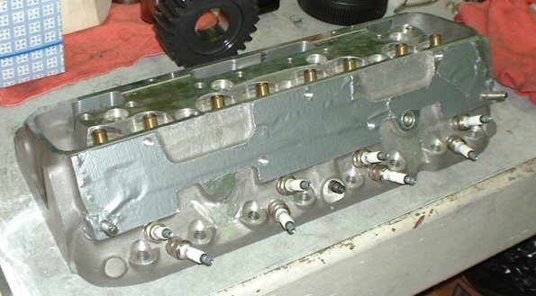
Figure 2: Band-Aid Cooling Fix for SBC Heads

The developers recognized the effects of those problems, without having access to the detailed combustion data we are talking about here. And by virtue of exhaustive experimenting and testing, they were able to go a long way toward solving the problems and producing excellent power results..

In order to try and equalize the performance of each cylinder, they developed (a) camshafts with 16 different lobes (profiles and / or centerlines) to attempt to equalize the VE in each cylinder, (b) bent distributor reluctor blades to provide different spark timing to compensate for the differences in mixture motion in various cylinders, and (c) wildly radical carburetor jetting to attempt to (1) equalize the mixture quality among the cylinders, and (2) to compensate for the centrifugal force generated in racetrack corners that moved the fuel away from the inner jets and toward the outer jets.

Continuing with that story (just because it is interesting), when GM developed the "SB-2" head (for NASCAR), they re-oriented the combustion chambers solely to improve the mixture-motion consistency for the central 4-barrel layout. The front pair of cylinders was symmetrical and the rear pair was symmetrical, but the front and rear pairs were mirror images ( valve sequencing of I-E-I-E-E-I-E-I ). That enabled the natural curvature of the intake runners to develop the mixture motion complimentary to what all the cylinders wanted, thereby reducing the combustion differences between the cylinders. It also increased the runner-length differences between the center and end cylinders. . However, it left in place the two adjacent center-cylinder exhaust valves, thereby keeping the middle-cylinder hotspot.

When GM developed the R-07 (4.500 inch bore center) NASCAR engine, they adopted a symmetrical cylinder layout (like the Fords had forever,) with a valve arrangement of I-E-I-E-I-E-I-E. That eliminated the center-cylinder hotspot, but made the problem of complimentary mixture motion worse on the rear two "driver-side" cylinders and on the front two "passenger-side" cylinders.

{ Personally, I think that if the R-07 had the SB-2 valve sequence along with the canted / offset valve and chamber layout, PLUS the inclusion of a generous coolant bay between the center two cylinder exhaust valves, it would have been optimal with regard to the mandated center 4-barrel manifolding. ]

COMBUSTION MYTHS

Here are a few commonly-believed Combustion Myths and the associated Realities, which were quantified by means of realtime in-cylinder and in-port pressure data.

1. MYTH: - - The trapped mass is ignited at the same crankshaft location every cycle;
   REALITY: The location of ignition can vary by 8-10 crankshaft degrees;
2. MYTH: - - Peak cylinder pressure occurs at the same crankshaft location every cycle;
   REALITY: Peak pressure location can vary by 10-15 degrees;
3. MYTH: - - Combustion on every cycle is identical;
   REALITY: Peak cylinder pressure in any one cylinder can vary by 300 psi from cycle to cycle;
4. MYTH: - - The majority of produced energy goes out the flywheel-end of the crankshaft.
   REALITY: At least 30% of energy produced goes out the tail pipe (and another large percentage goes out the cooling system).

It is interesting to note that today's production vehicles are so efficient in terms of consuming all the trapped mass each cycle that when operating on a stoichiometric air / fuel ratio, typically 96% to 98% of the trapped mass is burned.

TECHNOLOGY DEVELOPMENT

It is safe to say that the major impetus for the science we know as “combustion analysis” came from the government’s mandates, beginning in the 1960’s, for (a) greater fuel economy and (b) for reduced emissions.

Pioneers in this field include Dr. Andrew Randolph (GM Research, Hendrick Motorsports, and currently Technical Director at ECR Engines) and Dr. Paulius Puzinauskas (Associate Professor, Univesity of Alabama).

Dr. Randolph did research work at General Motors that resulted in the production of several groundbreaking SAE Technical Papers (including 900170, 900171, 942487, and 942488). Those papers are a rich source of detailed analysis and insights into the collection and interpretation of cylinder pressure data, and are highly recommended reading for anyone having a deeper interest in this subject.

AT A BARE MINIMUM, I recomend reading Dr. Randolph's SAE paper (942488) entitled Optimizing Race Engine Performance One Cylinder at at Time.

Other highly recommended reading on this subject include Dr. Puzinauskas' SAE papers 920808 (Characterizing Engine Knock) and 941881 (Measuring Intake Pressures), and Mendera, Spyra and Smereka on the Analysis to Determine Mass Fraction Burned ( ISSN 1231-4005).

During the development of the Saturn Inline-4 (SOHC and DOHC) in the late '80s and early '90s, Dr. Randolph and his team discovered that engines from the production environment didn’t work the same way as engines developed in a lab environment, so they moved their analysis tools from the lab into the production environment.

As a result, Dr. Randolph introduced an engineering-driven process to develop the lightweight 2v and 4v Saturn production engines to where they had good fuel specifics, good emissions (for the time), and produced 60+ HP per liter (as compared, for example to the heavy, fuel-hog, 35 hp per liter “Iron Duke” engine).

The combustion improvements which led to the achievement of the government emissions and economy mandates (a more homogeneous mixture development and distribution, a faster and more homogeneous burn, fewer unburned byproducts, fewer misfires, and more consistent cycle-to-cycle performance) can also be applied to the goal of making MORE POWER.

In fact, the science of combustion analysis has been instrumental in the development of the NASCAR CUP engines (naturally-aspirated, iron block, single 4-barrel [carburetor or throttle body], 2-valve, pushrod, 358 cubic inches) to where, at the end of 2014, they produced over 890 HP at over 9000 rpm for hours at a time.

(Of course, that power level was reached just prior to NASCAR's dimwitted 2015 "tapered spacer" rule)

INSTRUMENTING THE ENGINE

The proper instrumentation of a cylinder head to obtain correct, instantaneous cylinder pressure can be a substantial challenge.

There are several requirements for successful sensor location:

1. The sensors must be located in a position and orientation that enables the collection of accurate data;
2. The cylinder and exhaust sensor feed passages must be quite small in order to prevent impingement of extremely hot gasses onto the sensor elements.
3. The passages must pass through solid portions of the cylinder head.
4. The sensors must be located in a position that allows them to be kept as cool as possible to provide the best possible accuracy and stability.

The following picture shows a contemporary R-07 head for a NASCAR CUP engine, which was fitted with a combustion analysis sensor suite (combustion chambers and intake ports, no exhaust sensing on this particular test setup).

The cylinder pressure and intake pressure taps are shown with brass rods through them to help visualize their locations and orientations. The 4mm cylinder pressure tap is located just under the spark plug bore and is parallel to the deck and close to water jacket in order to achieve optimal cooling. The outer portions of both these taps are threaded and spotfaced to accept the appropriate piezoelectric sensors.

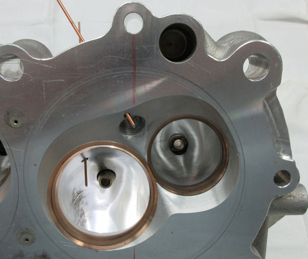
Figure 3: Instrumented Cylinder Head

The term PEGGING refers to the essential process of referencing the output of a transducer to a known basis, or reference value, provided by one or more dedicated transducers. The reference pressure provides a basis by which a critical transducer's output can be normalized to the internal engine environment.

Typically, the pegging sensor is a block-mounted piezoresistive sensor at bottom of the bore to provide pegging at BDC, which is the favored methodology (as long as one can fit the sensor into the block). In addition, that pegging sensor gives insight into what is happening in the crankcase with regard to such parameters as ring seal, windage, and crankcase pumping pressures.

Dr. Randolph's SAE paper 900171 presents a detailed discussion of pegging methods and data analysis.

SENSOR CHALLENGES

It goes without saying that the effective analysis of in-cylinder pressure data depends on the accuracy of the raw cylinder pressure dataset. Therefore, the technology developers have gone to great lengths to find techniques that minimize the errors that occur in the measurements.

Those techniques include:

1. data-stream digital filtering,
2. protecting sensors from thermal shock,
3. shielding sensors from electrical interference such as RFI from ignition components, ground noise, etc;
4. protecting sensors from structural vibrations in the engine components from sources such as high-velocity valve-closing events, and others.

Crankshaft position encoding at high frequencies places a big demand on the shaft encoders when they are operating near their rated frequency capacity. Further, the encoder is prone to vibration failure.

Thermal shock at the face of the cylinder pressure transducer is a major problem. Dr. Randolph's SAE paper 900171 presents an analysis of the techniques for mounting cylinder pressure transducers to maximize data accuracy.

Shielding the piezorestive cylinder pressure sensors from combustion temperatures involves a complex array of tiny holes and annuli. The problem is to determine the proper sizes and arrangements of these shielding holes and the metallurgical properties of the shield component. Those parameters are critical to obtaining accurate data without introducing a meaningful phase lag due to pressure wave restriction in too-small a hole. (I have been told that currently, (2020), most combustion sensor manufaturers incorporate "flame guards", which are steel caps containing an array of tiny holes that snap onto the face of the sensor.)

The proper shielding techniques increase the Helmholtz frequency to more than 10x higher than the low-pass filter in the channel, therefore passage-induced resonance is avoided.

Obviously the dedicated cylinder pressure sensors (Kistler et al) require some precise machining in the engine, and the location of a sensor could easily be compromised by the absence of solid material to drill through (no drilling through waterjackets, please). The positioning shown in Figure 2 is ideal.

SPARK PLUG PRESSURE SENSORS

The sensor port drilling methodology shown in Figure 2 is not always an option. For those instances, there are the $3000 spark plugs (Spark Plug Sensors, or SPS). They are combustion pressure transducers that have been modified to include the function of a spark plug.

But there are known compromises in the use of SPS. The pressure sensing element is a 2mm diaphragm, and the modifications necessary to insulate the sensor from the voltage transients that occur during spark generation degrade the sensing accuracy.

Further, running at full power settings with SPS can put the program at risk because (a) the sparkplug tip is not the same configuration as what would be used in competition (compromised data), and (b) the heat ranges available do not provide the very cold plugs typically required for sustained high power operation, so it can be difficult to avoid pre-ignition with SPS.

What are sparkplug sensors adequate for?  With correct interfacing, they are adequate for net IMEP. They are adequate for approximating the 50% Mass Fraction Burned (MFB) point, but the diameter and length of the tiny orifice leading up to the crystal sensing element affects sensor response time and signal phase shift.

 SPS peak pressure measurements are not suitable for individual thermodynamic heat release calculations, and SPS are not good for sensing low pressures and deltas, so the determination of pumping MEP is not ideal. Significant temperature changes and thermal shock degrade their accuracy.

In summary, SPS are a reasonable compromise if and when thereare no other options.

COLLECTING THE DATA

The current systems in use in NASCAR engine companies have been developed and refined to the point that every 1/10 degree of crankshaft rotation at 10,000 rpm, they can capture instantaneous (a) cylinder pressure, (b) intake port pressure, (c) exhaust port pressure from all 8 cylinders, plus crankshaft position and various environmental variables, and 8 cylinders of EGT, albeit at a much slower rate because EGT sensors that can survive in that environment have a much slower response..

Think about that.

That data capture capability requires a substantial amount of (a) processor resource, (b) memory resource, (c) input bandwidth, and (d) sophisticated software.

Consider first the input requirements. Capturing data every 1/10 of a degree means 3600 readings from EACH CHANNEL every revolution. Ten-thousand rpm is 167 revolutions per second, so to get 3600 readings during 167 consecutive revolutions at 10,000 rpm requires over 600 KHz of conversion bandwidth per Analog-to-Digital (A/D) channel.

In order to capture the data items described above, an 8-cylinder engine requires 3 fast channels per cylinder plus several more fast channels for pegging (reference) pressures and crankshaft position, plus some slower channels for EGT and environmental temperatures.. So 36 channels is a reasonable estimate for a system.

If we assume each channel has a 12-bit A/D converter, (which provides 1 in 4096 granularity, or 1.2 millivolts on a 5v signal), the DMA data rate into the system memory must be at least 43.3 megabytes per second.

( If the system used 16-bit A/D converters, the input DMA bandwidth would not change, since a 12-bit quantity and a 16-bit quantity both occupy 2 bytes of memory. However, a granularity of 1 part in 65536 seems to be a bit of overkill.)

So a test that spans 300 consecutive cycles on an 8-cylinder engine, instrumented as described, would produce a dataset of at least 52 megabytes at a data rate of at lease 29 megabytes per second. Fortunately, that is not terribly challenging for today's memory systems.

DATA REDUCTION AND PRESENTATION

Collecting and storing the data from a test is only the beginning. When the data gathering is complete, an array of massively complex software is used to analyze the mountain of information and reduce it to an intelligible form of graphs and tables.

In the past, data that was taken every 1 degree of crankshaft rotation data was considered sufficient. Now the standard is 1/10 degree. One immediately asks: What changed to make that order-of-magnitude increase in bandwidth necessary?

Several things. First, 1/10-degree data provides the ability to examine what is going on in greater detail. For example, MBT Timing (Minimum Spark Advance to achieve Maximum Torque, or Min Best Torque Timing, MBT} is always being sought for each individual cylinder. With 1 degree data, MBT can only be determined with 1° resolution. Today, with 1/10-degree data, MBT is determined within 3/10 of a degree.

Second, higher data rates are very valuable in sensing incipient auto-ignition ("detonation"). The primary acoustic knock frequencies in engines with 4-inch+ bores are around 6 kHz, but they are much higher in 3-inch bore 4-cylinder engines, so the higher rates are needed to capture the 2nd and 3rd mode signals for good signal-to-noise ratios.

Although it is generally accepted that 1.0 degree resolution can provide adequate data, it is likely to be quite noisy, so some flitering is required. Any realtime filtering techniques inserts a phase lag into the data. For example, if one uses a 7-point polynomial-fit filter on 1 degree data, the results are probably 'OK", but the polynomial-fit method requires a great deal more real-time processing resource. Using a 7-point-wide travelling avarage window is simpler, but it adds a 7-point lag to the data. Capturing 1/10 degree data is more hardware intensive, but the 7-point lag from using the travelling average method on 1/10 degree data gives good smoothing without the phase shift and required much less processor resource.

COMBUSTION ANALYSIS RESULTS

This section shows examples of the Combustion Analysis graphics, with a brief commentary on their uses.

There is a wide variety of graphs and tabular data that can be provided by the processing software. Some (but not all) of those presentations (both graphical and numerical) include:

1. Crankshaft rotation angle at which 10%, 50%, and 90% of the charge has been burned (mass-fraction-burned, MFB);
2. PV diagrams for each cylinder focused on pumping loop losses;
3. Peak cylinder pressure value for each cylinder across several consecutive cycles;
4. Peak cylinder pressure location for each cylinder across several consecutive cycles;
5. MBT timing for each cylinder;
6. Indicated MEP (IMEP), Pumping MEP (PMEP) and Net MEP of each cylinder across several consecutive cycles
7. Intake and exhaust port pressures;

Those data and graphs help isolate deficient portions of the engine and provide insight into what changes might improve engine performance.

Figure 3 shows a plot of cylinder pressure vs. crankshaft angle for one cycle on a high performance engine. This plot is exactly the same concept as is shown in Figure 1 above, but it shows a single cycle of an engine operating at a high BMEP, whereas Figure 1 shows data aggregated from a large number of cycles superimposed on each other.

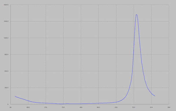
Figure 4: Cylinder Pressure vs. Crankshaft Angle

It is more convenient to extract meaning from the same data presented in a different format. Instead of plotting pressure vs. crank rotation, a simple calculation can transform the X-axis from crankshaft position into cylinder volume, thereby presenting the pressure vs. cylinder volume (PV) diagram. Figure 5 is the PV-format presentation of the same data shown in Figure 4.

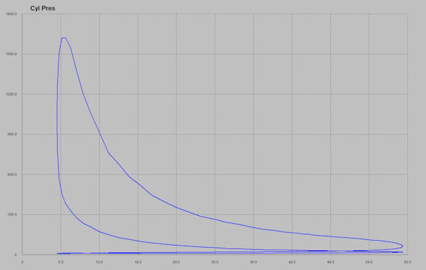
Figure 5: PV (pressure-Volume) Diagram

PV diagrams and combustion thermodynamics are explained in thorough detail in C.F.Taylor (ref:5:2:107-146)

A quick glance at Figure 5 shows that the compression and expansion cycles are well-presented, but the (critical) pumping loop is obscured by the scaling. Figure 6 shows an expanded look into the pumping portion of the cycle, from which some helpful information about power losses can be extracted. (The valve events in the picture are not exact representations of those in the engine depicted, but are merely to help identify regions of interest on the curve.)

Note how the cylinder pressure around IVO in this diagram is quite low, which assists in getting the fresh charge moving into the cylinder. However, the cylinder pressure up through most of the exchaust stroke suggest there might be some unwarranted restriction in the exhaust circuit. The cylinder pressure begins to rise in the region of peak piston velocity on the intake stroke and continues to rise through BDC, suggesting the existence of some effective intake ram tuning.

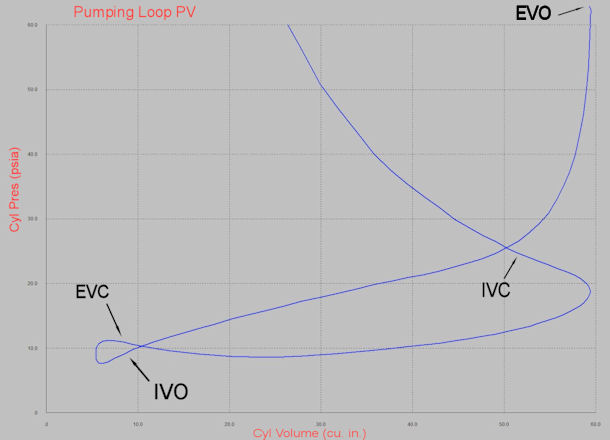
Figure 6: PV Pumping Loop

A further reformatting of the PV data provides a diagram that (a) shows both the pumping loop and the work loop effectively, and (b) in which the compression and expansion cycles tend to be mostly straight lines, the slopes of which are useful for heat release and thermodynamic calculations.

This reformatting presents the data in a logarithmic form, in which the X-axis is the logarithm of cylinder volume and the Y-axis is the logarithm of cylinder pressure. The "log-log" presentation is preferred by many engineers. Figure 7 shows a comparison of the same data in both formats.

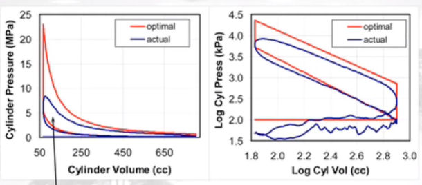
Figure 7: PV Diagram in Linear Scale and Log-Log Scale

Next, when we display intake and exhaust port pressures and velocities with the cylinder pressure data, some valuable insights about camshaft lobe timing and port runner dynamic pressure tuning become visible. Figure 8 shows that plot for the example engine at 3300 rpm.

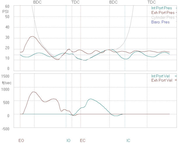
Figure 8: 3300 RPM Cylinder Pressure with Port Pressures and Velocities

Note how both the intake and exhaust flows reverse around TDC, and how the intake reverses again after BDC. The causes of those events are shown by the intake and exhaust pressure curves.

For comparison, Figure 9 shows the same data for the same engine at its torque peak (4800 rpm). Note how the flow velocities in both ports are higher and there are no flow reversals in either port. Note also how the third reflection of the intake pulse coincides with IVO.

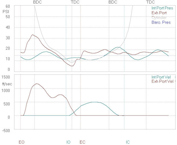
Figure 9: 4800 RPM Cylinder Pressure with Port Pressures and Velocities

The following plots, provided courtesy of iSystems Performance Inc, show actual Peak Pressure data, Mass Fraction Burned (MFB) data, and Air to Fuel Ratio (AFR) data from a test of a 6-cylinder "High Performance" Porsche engine, taken over 50 consecutive cycles at WOT.

At first glance, they look like the products of a random-number generator. However, they illustrate the substantial differences in performance and consistency of each cylinder.

The measurement of peak cylinder pressure VALUE and peak cylinder pressure LOCATION, and the variances from cycle to cycle play an inportant part in evaluating how well the engine is operating.

Figure 10 shows the cycle-to-cycle variation in the VALUE ( in psi ) of peak cylinder pressure. Note how cylinder #2 (lighter orange) is clearly outperforming all the others, and how cylinder #5 (light grey) is significantly underperforming..

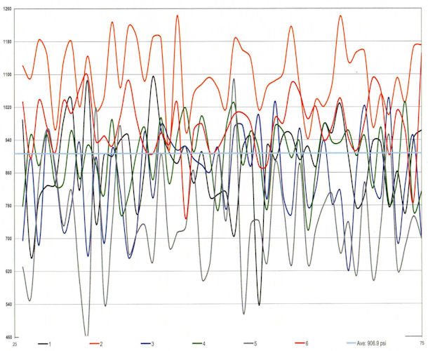
Figure 10: Peak Pressure VALUE (PSI) over 50 Consecutive Cycles, All 6 Cylinders
(Courtesy of iSystems Performance)

Figure 11 shows the large cycle-to-cycle and cylinder-to-cylinder variation in the LOCATION (crank degrees ATC) of the peak cylinder pressure (same engine, same run). Note here that cylinder #2 (light orange) is the best performer while cylinder #5 (light grey) is clearly the worst.

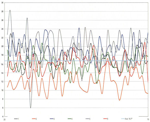
Figure 11: Peak Pressure LOCATION (Crank Degrees ATC) over 50 Consecutive Cycles, All 6 Cylinders
(Courtesy of iSystems Performance)

The determination of the crankshaft angles and variations at which certain percentages of the combustible mass have been burned (MFB) provides valuable insights into the combustion process itself.

The consistency of ignition and the rate of burn in a given cylinder is shown by the displays of crank angles for the "start" of combustion (10% MFB), the "middle" of combustion (50% MFB), and the "end" of combustion (90% MFB).

There were some older studies showing that the location of the 50% MFB point at 8 degrees ATC corresponded to the optimal ignition point. More current developments indicate that 50% MFB at 5 degrees ATC is even better..

I would like to have presented plots of 10% and 50% MFB from the same dataset as the other graphs here, but those two charts were not available to me.

Figure 12 shows the locations of the 90% MFB point over 50 consecutive combustion cycles for all 6 cylinders on the same engine. Again, cylinder #2 (light orange) has the fastest burn and probably the earliest ignition, while again, cylinder #5 is lagging the pack.

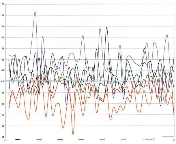
Figure 12: 90% MFB Location over 50 Consecutive Cycles, All 6 Cylinders
(Courtesy of iSystems Performance)

Figure 12 shows the variation in Air-Fuel ratio in the same engine over a WOT range of 4500 to 7500 rpm. The wild fluctuation and range of AFR (12.0 to 14.18) shows that there are some serious problems with fuel delivery and / or mass airflow variation.

Quoting from Dr. Randolph:
"It is very difficult to get uniform fuel distribution in a highly-tuned engine with port injectors.  Of course, in NASCAR Cup engines the situation is aggravated further with the injector mounting mandated in the individual runners, not the individual ports.  Worse yet, the injectors by rule must be mounted vertically (perpendicular to the runner floor) such that the fuel simply sprays on the runner wall, not directed toward the intake valve."

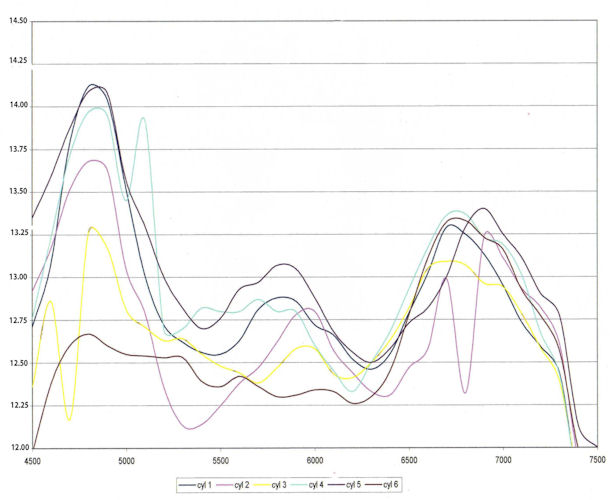
Figure 13: Air-Fuel Ratio Variation from 4500 to 7500 RPM, All 6 Cylinders
(Courtesy of iSystems Performance)

INTERPRETATION and APPLICATION

Once you have the ability to gather, analyze and correctly interpret the real time data, the next question is: OK, how do I fix the engine in order to reduce the variability from cycle to cycle and from cylinder to cylinder?.

Of course, the ideal goal is to achieve a "flatline" on the critical parameters (peak pressure value and location, 10, 50 and 90 MFB points) by fixing air massflow distribution, fuel distribution, mixture homogeneity, in-cylinder mixture motion, individual spark timing, and other variables.

Again, quoting Dr. Randolph:
Cup engines are atypical because the combination of a maximum 12.0 compression ratio and high-octane fuel (partly due to the wonders of ethanol) eliminates the possibility of knock (or autoignition).. Most consumer and race engines must have retarded ignition under some operating conditions (typically low speed, high load) due to knock concerns, thus retarding all of the combustion metrics".

Regrettably, complete flatlining does not occur, but the more one can reduce those variations, and make all cylinders operate with similar pressure curves, the more power the engine will produce and the more efficiently it can be made to operate.

The contemporary standard for "flatlining" is to achieve a coefficient of variation (COV) on IMEP of 2%.

 CONCLUSION

This article is only intended as a skimpy introduction into the science of Combustion Analysis. The current literature is rich with new and more detailed information on current technology and discoveries.

Again, I want to recomend reading Dr. Randolph's SAE paper (942488) entitled Optimizing Race Engine Performance One Cylinder at at Time.

And one closing thought: before one begins to apply Combustion Analysis to an engine, the engine should already be optimized by the normal methodologies.